Instructions

1.1 Fit data - how to upload data files

When we click on the Fit data tab, a page opens asking us to upload a file. To upload a file, we click Browse and select the desired .csv file from our computer.
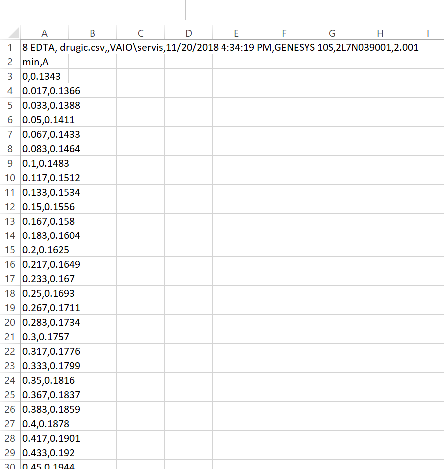
The file must be in .csv format and have values for time and absorbance in the form of a single column separated by a comma [min, A] (download example). The first line (cell A1) of the .csv file must contain text (e.g. the name of the file; any text suffices) and the second line must be min,A (cell A2). (see example photo).
All other lines must consist of time and absorbance data. No spaces between characters are allowed; no other text apart from the one mentioned above may be present. This format for time-concentration .csv files is created by default by the VisionLite Genesys software; users who have other software for recording progress curves might need to modify their files before uploading them to iFIT.
Once we have uploaded the desired data, we click on the Submit , which redirects us to the interface for determining the range parameters. If the above conditions are not fulfilled, the program notifies us with the message Wrong file format, please upload .csv file.

1.2 Range parameters - how to crop the progress curve

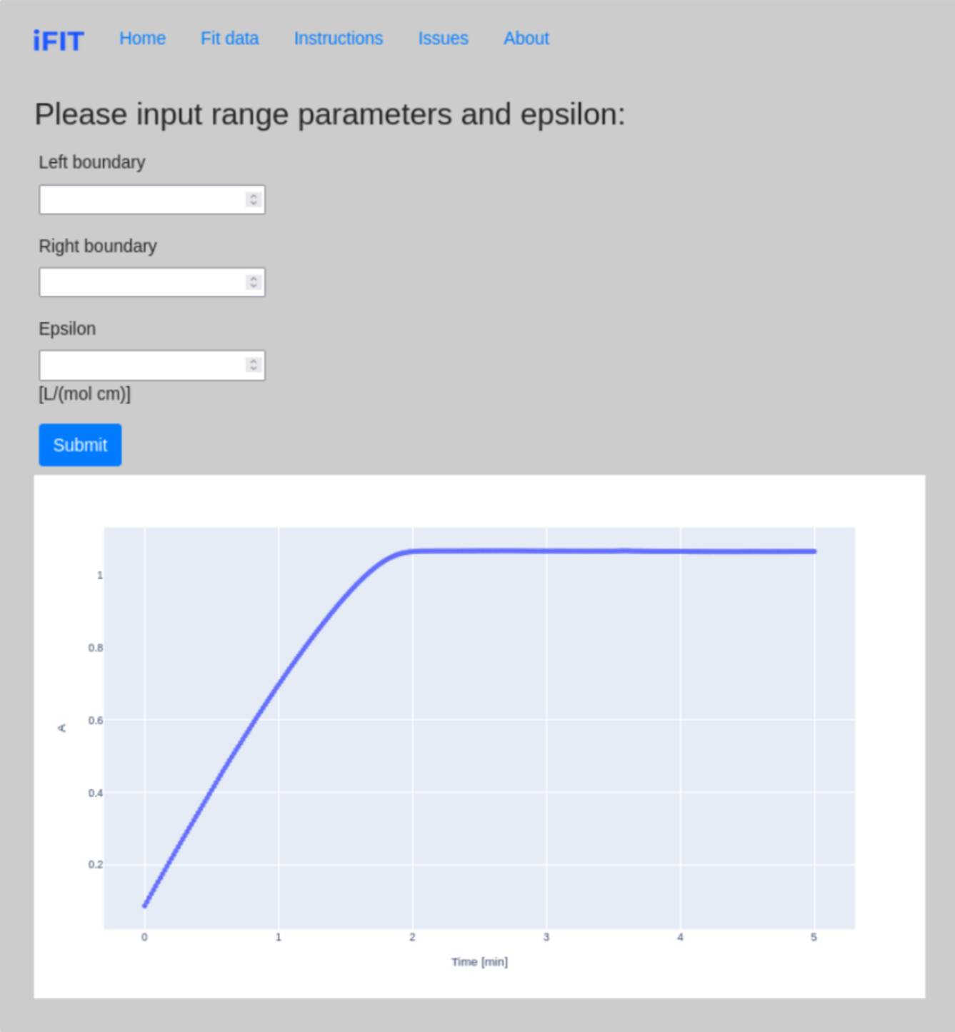
At this step, we define range parameters for progress curve fitting. Left boundary and Right boundary refer to the part of the progress curve that is initially fitted with the integrated Michaelis-Menten equation. E.g., if the progress curve terminates at 5 minutes and we only want to use the first three minutes of recorded data, we input 0 for Left boundary and 3 for Right boundary; we do this when the early part of the curve, or the plateau, contain so much noise that the integrated Michaelis-Menten equation might not be able to calculate a value for Michaelis constant K_M and limiting rate V_MAX.
Epsilon (ε) is the molar extinction coefficient for the product of the reaction, a measure of how strongly a chemical species or substance absorbs light at a particular wavelength. If your absorbance data has already been converted into molar concentration units, input 1 for epsilon, for milimolar concentration input 1000 for epsilon, etc.
At the end of the page, a graph with data is drawn, which can be moved, cut, "zoomed", etc.
When you have finished defining the parameters, click the Submit button.

1.3 Initial parameters - how to determine initial parameter estimates

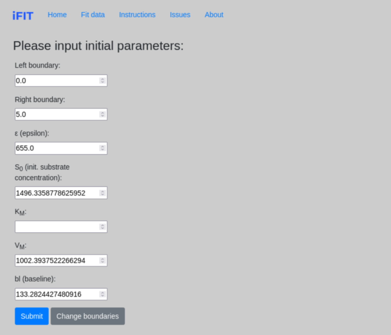
Once we determine the range parameters, the program calculates initial estimates for most of the parameters that are required for further fitting. However, we need to determine an estimate for the parameter K_M ourselves. The field K_M should not be left blank and must always be filled with numerical values.
The true initial substrate concentration S₀ is calculated only when the time interval from zero to the point on the curve where the entire substrate is consumed in the reaction is selected (see 1.2 Range parameters). Otherwise, the calculated value ​​will be incorrect.
On this subpage, we have the option to change the boundaries of our “fit” by clicking Change boundaries, which redirects us to the previous page.

1.4 Final plots - the final result

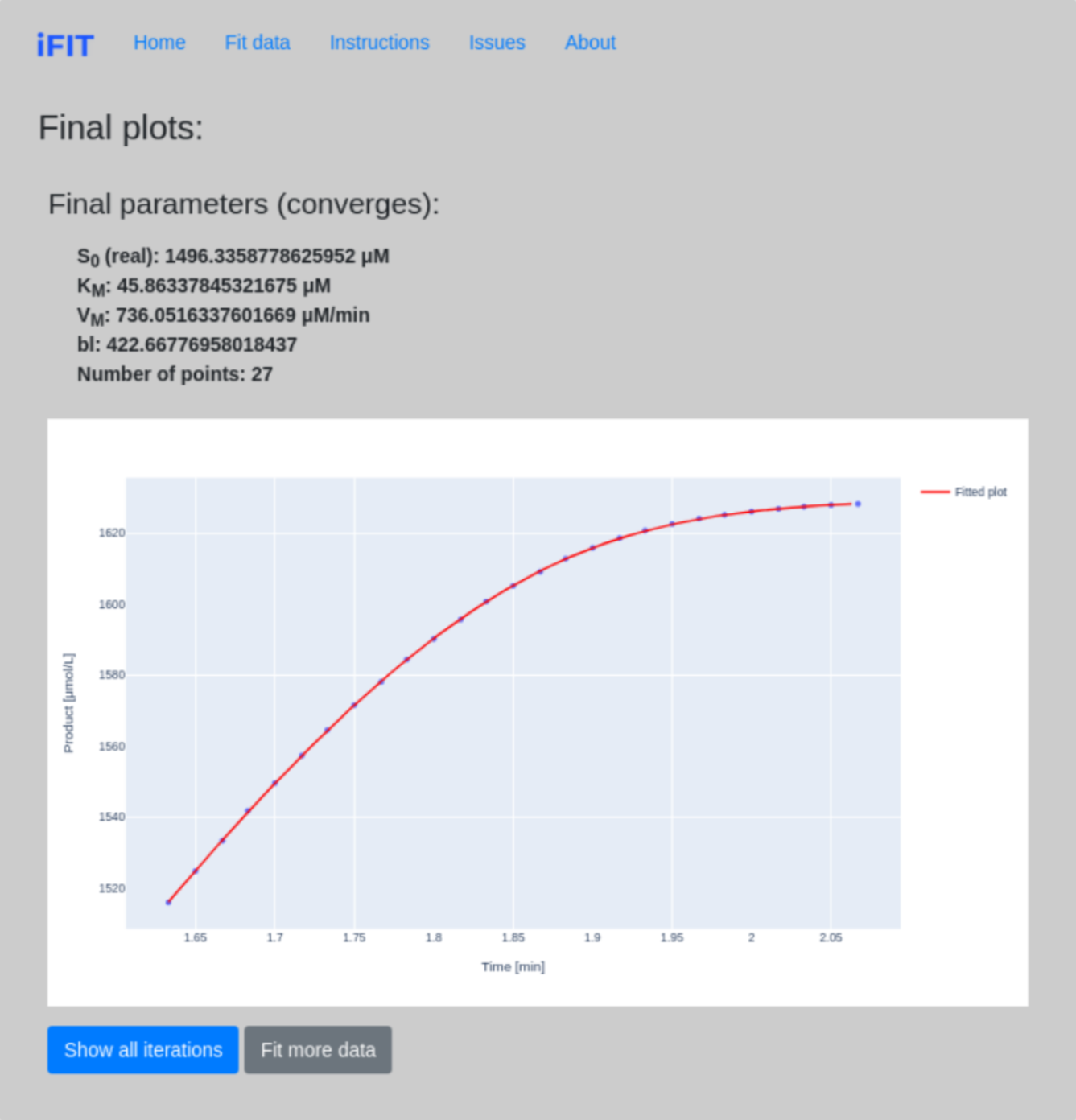
Here, the application displays all the final parameters of our fit and draws a graph that can be saved by clicking on the Camera icon. In addition, the program can print and draw the whole fitting process. To do this, click on Show all iterations. If you want to fit more data, click on Fit more data.
If it turns out that the fit does not converge (i.e., the program oscillates between two or more values), this is displayed, and we can also see all the iterations, with their calculated parameters of K_M and V_MAX.

1.5 Troubleshooting

We recommend troubleshooting for problems that are critical to normal iFIT operation and might impact your experience.
See here: iFIT Troubleshooting.